Tutorial · Anti-collapse regularization ·
SIGReg from First Principles
A step-by-step construction of an anti-collapse regularizer for JEPAs, from characteristic functions through the Cramér–Wold theorem to a working training loop.
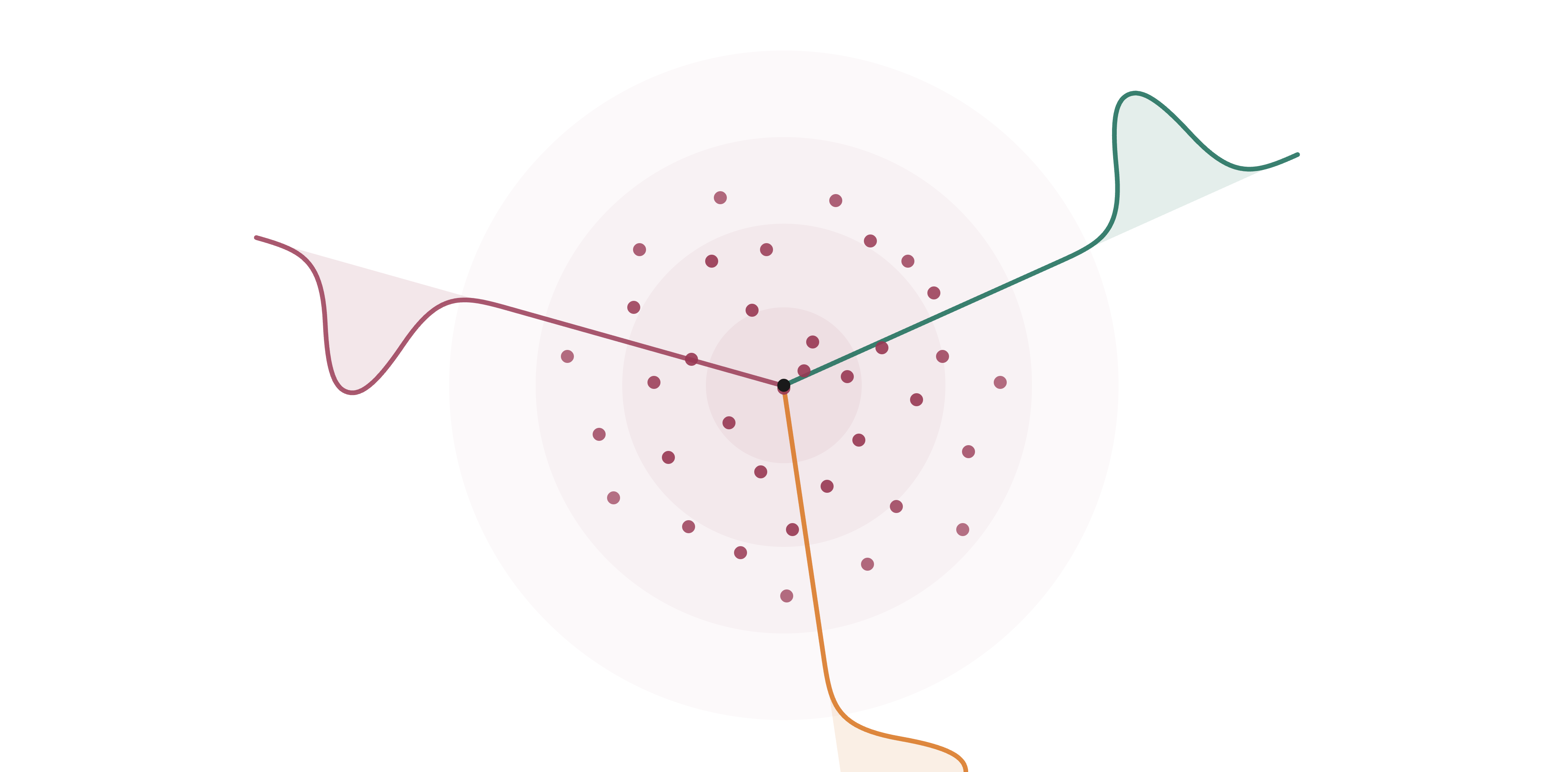
Scope. SIGReg was introduced in LeJEPA as a general anti-collapse regularizer for joint-embedding predictive architectures. This tutorial develops SIGReg in that general setting and uses LeWorldModel (LeWM) as one concrete temporal-prediction application.
§1. The problem we're solving
SIGReg belongs to the general JEPA setting introduced in LeJEPA. It starts with two related views, $x$ and $x^+$: they may be two crops of an image, a visible and masked region, adjacent video frames, two sensor modalities, or anything else that shares semantic information. A shared encoder maps them to embeddings and is trained to make one embedding agree with the other.
In the LeWM setup, there are three components. An encoder $\text{enc}_\theta$ maps an observation $o$ (an image, sensor reading, or state vector) to an embedding $z \in \mathbb{R}^D$. A predictor $\text{pred}_\phi$ maps a current embedding $z_t$ to a predicted next embedding $\hat z_{t+1}$. The predictor is action-conditioned, $\hat z_{t+1} = \text{pred}_\phi(z_t, a_t)$, since predicting the next state of the world generally requires knowing the action taken. This is what makes the learned model usable for planning. (We suppress the action $a_t$ throughout this tutorial because neither SIGReg nor the collapse argument depends on it.)
A prediction loss then compares the predicted next embedding with the actual encoded next observation, $z_{t+1} = \text{enc}_\theta(o_{t+1})$:
$$\mathcal{L}_{\text{pred}} = \big\|\hat z_{t+1} - z_{t+1}\big\|^2.$$
The catch lies in the loss and the diagram. Both sides of the loss pass through the same encoder. The trivial solution $\text{enc}_\theta(o) = c$ (a constant function that maps every observation to the same point) gives $z_t = z_{t+1} = c$, and any predictor that outputs $c$ achieves $\mathcal{L}_{\text{pred}} = 0$ exactly. The loss is perfectly minimized, but the encoder has thrown away every bit of information about the input. The world model is useless for any downstream task.
This is representational collapse, and it isn't a hypothetical risk: training LeWM on $\mathcal{L}_{\text{pred}}$ alone can converge to trivial encoders. Gradient descent takes the easiest path to zero loss, and "encode everything the same" is the easiest path.
The need for a regularizer
The natural way to prevent collapse is to add a regularizer term $\mathcal{R}(Z)$ that penalizes the encoder when its output distribution is trivial: concentrated, low-rank, or low-variance. To build an actual loss, however, we need a concrete non-collapsed target and a differentiable way to measure whether the batch has reached it. SIGReg makes that target explicit: the batch distribution should match the standard isotropic Gaussian $\mathcal{N}(0, I_D)$.
In the training loop, the total loss becomes
$$\mathcal{L}_{\text{total}} = \mathcal{L}_{\text{pred}} + \lambda_{\text{reg}} \cdot \mathcal{R}(Z)$$
where $Z = \{z_1, \dots, z_N\}$ is the batch of embeddings. For SIGReg's version of $\mathcal{R}(Z)$ to do its job, it needs three concrete properties.
First, zero in the ideal population limit when $Z$ follows $\mathcal{N}(0, I_D)$, positive otherwise. This is the SIGReg-specific target, not a requirement every anti-collapse method must satisfy. If SIGReg vanished for some non-Gaussian population distribution, it would fail to detect that deviation and the corresponding collapse mode could sneak through. Conversely, if it stayed positive for the target Gaussian distribution even in the ideal limit, it would wrongly punish the distribution it is designed to enforce. With finite batches, the empirical loss should be small rather than literally zero.
Second, differentiable in $Z$. Gradient descent can't use it otherwise. This immediately rules out the classical statistical Gaussianity tests. Kolmogorov–Smirnov uses a supremum over CDFs, and Shapiro–Wilk uses sorted order statistics; neither operation has usable gradients.
Third, scalable to high $D$ and modest batch sizes. Embedding dimension is on the order of hundreds (the LeWM paper uses $D = 192$) and batch sizes are on the order of hundreds. The per-step cost should be at most linear in $D$ and $N$; we can't afford anything that scales as $D^2$ or $N^2$ given that this term is evaluated at every training step.
Two design choices are implicit in SIGReg but worth naming. $\mathcal{R}$ acts on a single batch of embeddings, with no negative samples and no paired contrasts. This distinguishes it from contrastive methods like SimCLR or MoCo. And the target is a known, parameterized distribution: the standard isotropic Gaussian, not the empirical distribution of some other batch or a learned reference.
Three flavors of Gaussian
The Gaussian family in $D$ dimensions splits by what its covariance matrix can look like:
Isotropic uses $\Sigma = \sigma^2 I_D$: one variance for every dimension, no correlations, and contours that are perfect spheres. Diagonal (anisotropic) lets each dimension have its own variance, $\Sigma = \text{diag}(\sigma_1^2, \dots, \sigma_D^2)$, so contours are axis-aligned ellipses but dimensions remain independent. Full covariance allows any positive-definite $\Sigma$, so contours can tilt and stretch arbitrarily, encoding correlations between dimensions.
Parameter count tells the same story: isotropic has $1$ free parameter, diagonal has $D$, full has $D(D+1)/2$. The isotropic case is the simplest and most symmetric, which is why it shows up so often as a default modeling choice: it's the noise model in diffusion models and VAEs, the prior in Bayesian linear regression, the proposal distribution in MCMC, and the initialization distribution for neural network weights. torch.randn and numpy.random.randn give you exactly an isotropic standard normal.
Why the isotropic Gaussian as target
SIGReg picks $\mathcal{N}(0, I_D)$ as the target distribution for $\mathcal{R}$. The LeJEPA paper gives the main reason: under broad downstream probing assumptions, isotropic Gaussian embeddings minimize worst-case prediction risk. The regularizer is therefore not merely trying to make the embedding cloud "look nice"; it is pushing toward a distribution that the LeJEPA theory identifies as optimal for later tasks.
For this tutorial, three geometric intuitions are enough to understand why that target also prevents collapse.
First, full rank by construction. The covariance is $I_D$, so all $D$ eigenvalues equal $1$. Collapse to a lower-dimensional subspace is impossible at the optimum, because the optimum is full-dimensional.
Second, no preferred direction. The distribution is rotationally symmetric: rotating $z$ doesn't change its probability. The encoder is free to put information into any direction of the embedding space without the regularizer biasing any particular axis. We don't want to bake assumptions about embedding-space geometry into the regularizer.
Third, maximum entropy for fixed second moment. Among all distributions with mean $0$ and covariance $I_D$, the Gaussian is the most "uninformative" shape. It has the highest entropy, so the isotropic Gaussian is the least-committal full-rank target compatible with those first two moments.
An obvious alternative that fails
Before the construction proper, it's worth seeing what doesn't work. The most natural-looking idea: at each training step, for every embedding $z_i$, draw a fresh target $z^*_i \sim \mathcal{N}(0, I_D)$ and add the regularizer
$$\mathcal{L}_{\text{naive}} = \sum_i \|z_i - z^*_i\|^2.$$
It looks reasonable: pull every $z_i$ toward a Gaussian sample, so over many steps the $z_i$'s should "look Gaussian," right? Take the expectation in the random target $z^*$ for a single point. Using $\mathbb{E}[z^*] = 0$ and $\mathbb{E}[\|z^*\|^2] = D$:
$$\mathbb{E}_{z^*}\big[\|z - z^*\|^2\big] = \|z\|^2 - 2\, z^\top \underbrace{\mathbb{E}[z^*]}_{=\,0} + \underbrace{\mathbb{E}[\|z^*\|^2]}_{=\,D} = \|z\|^2 + D.$$
Differentiating in $z$:
$$\nabla_z\, \mathbb{E}_{z^*}\big[\|z - z^*\|^2\big] = 2z.$$
The gradient in expectation points from $z$ straight back to the origin, regardless of which $z^*$ was drawn. The random targets average out; what's left is a pure pull toward zero. That's exactly the collapse we wanted to prevent.
The conceptual mistake is conflating "samples from $\mathcal{N}(0, I)$" with "the distribution $\mathcal{N}(0, I)$ itself." We don't want any single $z_i$ to equal any particular sample. We want the empirical distribution of $\{z_1, \dots, z_N\}$ to be statistically indistinguishable from samples drawn from $\mathcal{N}(0, I)$. That's a property of the collection, not of individual points. The rest of this tutorial is about how to make "the collection looks Gaussian" into a single differentiable scalar.
So the question this tutorial answers is: how do you build a differentiable, sample-only function $\mathcal{R}(Z)$ whose population optimum is the isotropic Gaussian $\mathcal{N}(0, I_D)$, and that scales to modern embedding dimensions and batch sizes? The construction is SIGReg, and the next sections build it piece by piece.
§2. Characteristic functions
The question we left §1 with was: how do you build a differentiable function whose population optimum is the isotropic Gaussian? The familiar tool for comparing distributions, Kullback–Leibler divergence,
$$\text{KL}(p_Z \,\|\, p_0) = \int p_Z(z) \log \frac{p_Z(z)}{p_0(z)}\, dz,$$
doesn't work for us. KL requires knowing the density $p_Z$ of the encoder's output distribution. We don't have $p_Z$; all we have is a batch of samples $z_1, \dots, z_N$. Estimating $p_Z$ from those samples is hard (high-dimensional density estimation) and the resulting estimate isn't a smooth function of the underlying samples that we can backpropagate through.
A different approach: rather than comparing densities, compare the Fourier transforms of the distributions. This Fourier transform is called the characteristic function (CF). It identifies the distribution just as well as the density itself, but is much easier to estimate from samples in a differentiable way.
Because characteristic functions are complex-valued, it is worth briefly refreshing the bit of complex-number geometry we will use: the unit circle and Euler's formula.
A brief complex-number primer
A complex number $a + bi$ is a 2D point with coordinates $(a, b)$, where $i = \sqrt{-1}$ is the imaginary unit. The real part is the horizontal coordinate, the imaginary part is the vertical. Multiplication by $i$ rotates a point 90° counter-clockwise: $i \cdot 1 = i$, $i \cdot i = -1$, $i \cdot (-1) = -i$, $i \cdot (-i) = 1$. Four steps get you back where you started.
The exponential of an imaginary argument has a beautiful geometric meaning, given by Euler's formula:
$$e^{i\theta} = \cos\theta + i\sin\theta.$$
Geometrically, $e^{i\theta}$ is the point on the unit circle at angle $\theta$, measured counter-clockwise from the positive real axis. At $\theta = 0$ it's the point $1$; at $\theta = \pi/2$ it's $i$; at $\theta = \pi$ it's $-1$; at $\theta = 3\pi/2$ it's $-i$. Its magnitude is always $1$ because $|\cos\theta + i\sin\theta| = \sqrt{\cos^2\theta + \sin^2\theta} = 1$.
For any real number $X$ and any real parameter $t$, the quantity $e^{itX}$ is a single point on the unit circle at angle $tX$. Different values of $X$ give different points; different values of $t$ rotate the points around the circle at different rates.
The characteristic function
The characteristic function of a real random variable $X$ is the expected value of $e^{itX}$, treated as a function of the real parameter $t$:
$$\varphi_X(t) \;=\; \mathbb{E}\!\left[e^{itX}\right].$$
It's complex-valued (the output is a 2D point) and takes a real argument. Geometrically: draw a random $X$ from the distribution, which gives you a random point $e^{itX}$ on the unit circle (at angle $tX$); the characteristic function $\varphi_X(t)$ is the expected value of those random points, weighted by the probability of each $X$.
For a continuous distribution with density $p_X(x)$, this is
$$\varphi_X(t) \;=\; \int_{-\infty}^{\infty} e^{itx}\, p_X(x)\, dx,$$
exactly the Fourier transform of the density $p_X$ (with the standard probability sign convention). When no density exists, the expectation definition above still works; it is the Fourier transform of the probability measure itself.
What $t$ means: the frequency interpretation
$t$ is not part of the data or part of the distribution. It's a knob you (the analyst) choose. Each value of $t$ assigns an angle $t \cdot X$ to the random variable, which controls how spread out the resulting unit-circle points end up. Small $t$ shrinks all angles toward $0$, packing the points near the position $(1, 0)$ on the circle. Large $t$ inflates the angles, scattering the points around the entire circle. Pairs of nearby $X$ values produce wildly different unit-circle positions because the same difference $\Delta X$ becomes a larger angular difference $t \cdot \Delta X$.
Take a small five-point sample $\{-2, -1, 0, 1, 2\}$ and plot $e^{itx_n}$ on the unit circle for two values of $t$:
This is why $t$ is called the frequency parameter. The complex exponential $e^{itx} = \cos(tx) + i\sin(tx)$ is literally a wave; $t$ is how fast the wave oscillates as you sweep through $x$. Higher $t$ = faster oscillation = higher frequency.
The whole CF $\varphi_X(t)$ (the curve traced as $t$ ranges over all reals) tells you about the distribution at every scale. Small $t$ probes the coarse, large-scale shape: where is the mean, what's the spread? Large $t$ probes fine, small-scale features: how does the density wiggle, what's in the tails? Reading the entire function $\varphi(t)$ gives the full frequency-by-frequency description of the distribution.
Taylor expansion near $t = 0$. A useful general fact: expanding $e^{itX}$ in a power series and taking expectations termwise,
$$\varphi_X(t) \;=\; 1 \;+\; i\mu\, t \;-\; \tfrac{1}{2}(\mu^2 + \sigma^2)\, t^2 \;+\; O(t^3),$$
where $\mu = \mathbb{E}[X]$ and $\sigma^2 = \text{Var}(X)$. Behavior near $t = 0$ is determined by low-order moments: small $t$ probes mean and variance, while larger $t$ engages higher-order features (skewness, kurtosis, fine shape).
Fourier uniqueness
The fact that makes CFs useful is Fourier uniqueness: two probability distributions are equal if and only if their characteristic functions are equal. Knowing the entire function $\varphi_X(t)$ over all real $t$ is equivalent to knowing the distribution of $X$.
This is a foundational result in Fourier analysis. The intuition is that Fourier transformation is invertible: the map “distribution $\to$ characteristic function” is a bijection. The CF is a complete fingerprint of the distribution: different distributions give different fingerprints, and matching fingerprints means matching distributions.
This is the property SIGReg exploits. If we can match the CF of our embedding distribution to the CF of $\mathcal{N}(0, I_D)$, then by Fourier uniqueness, the distributions must match.
Worked example: the fair coin
Before turning CFs into a loss, it helps to look at a few fingerprints. Even tiny distributions leave recognizable patterns in their characteristic functions: a fair coin, a biased coin, and a Gaussian all produce different curves. The point of the example is not the coin itself; it is that studying the CF makes distributional differences visible.
Take $X$ to be a fair coin flip, equal to $0$ or $1$ each with probability $1/2$. Its characteristic function is
$$\varphi_X(t) \;=\; \mathbb{E}\!\left[e^{itX}\right] \;=\; \tfrac{1}{2}\, e^{i \cdot t \cdot 0} \,+\, \tfrac{1}{2}\, e^{i \cdot t \cdot 1} \;=\; \tfrac{1}{2}\big(1 + e^{it}\big).$$
So $\varphi_X(t)$ is the midpoint of two unit-circle points: $1$ (the point at angle $0$) and $e^{it}$ (the point at angle $t$).
To get the magnitude $|\varphi_X(t)|$, expand using Euler's formula and apply the magnitude formula $|a + bi|^2 = a^2 + b^2$. This is just trig identities applied carefully. Step by step:
Step 1. Expand $e^{it}$:
$$\varphi_X(t) = \tfrac{1}{2}(1 + \cos t + i \sin t).$$
Step 2. Identify real and imaginary parts:
$$\varphi_X(t) = \underbrace{\tfrac{1 + \cos t}{2}}_{\text{real part}} \;+\; i \cdot \underbrace{\tfrac{\sin t}{2}}_{\text{imaginary part}}.$$
Step 3. Apply $|a + bi|^2 = a^2 + b^2$:
$$|\varphi_X(t)|^2 = \left(\tfrac{1 + \cos t}{2}\right)^2 + \left(\tfrac{\sin t}{2}\right)^2 = \frac{(1 + \cos t)^2 + \sin^2 t}{4}.$$
Step 4. Expand $(1 + \cos t)^2 = 1 + 2\cos t + \cos^2 t$ and use $\cos^2 t + \sin^2 t = 1$:
$$|\varphi_X(t)|^2 = \frac{1 + 2\cos t + 1}{4} = \frac{1 + \cos t}{2}.$$
Step 5. Apply the half-angle identity $1 + \cos t = 2\cos^2(t/2)$:
$$|\varphi_X(t)|^2 = \cos^2(t/2) \quad\Longrightarrow\quad |\varphi_X(t)| = \big|\cos(t/2)\big|.$$
Sanity check at three obvious values of $t$:
- $t = 0$: $|\cos(0)| = 1$. Both unit vectors coincide at $(1, 0)$, midpoint magnitude is $1$. (This is $\varphi(0) = \mathbb{E}[1] = 1$, always true for any CF.)
- $t = \pi$: $|\cos(\pi/2)| = 0$. The two vectors are $1$ and $e^{i\pi} = -1$, diametrically opposite, midpoint is exactly the origin.
- $t = 2\pi$: $|\cos(\pi)| = 1$. The second vector has gone once around the circle and rejoined the first.
So $|\varphi_X(t)|$ oscillates between $0$ and $1$ with period $2\pi$ and never decays. This is the signature of a discrete distribution: its characteristic function may have zeros, as the fair coin does at $t = \pi$, but it keeps oscillating instead of settling toward $0$ as $|t|$ grows.
A geometric derivation
There's a one-line geometric picture for $|\varphi_X(t)| = |\cos(t/2)|$. The value $\varphi_X(t)$ is the midpoint of two unit vectors $A = 1$ and $B = e^{it}$, separated by angle $t$ at the origin. The triangle $(O, A, B)$ is isoceles with two sides of length $1$ and angle $t$ between them at $O$:
From fair to biased
The fair coin's CF is a limiting case of a more general fact. Take a biased coin with probability $p$ of getting $0$ and $1-p$ of getting $1$:
$$\varphi_X(t) \;=\; p + (1-p)\,e^{it}.$$
The same algebra as the fair case gives the result: expand with Euler, apply $|a+bi|^2$, and simplify.
$$|\varphi_X(t)|^2 \;=\; p^2 + (1-p)^2 + 2p(1-p)\cos t.$$
Use $p^2 + (1-p)^2 = 1 - 2p(1-p)$ and the identity $1 - \cos t = 2\sin^2(t/2)$:
$$\boxed{\;|\varphi_X(t)|^2 \;=\; 1 - 4p(1-p)\sin^2(t/2)\;}$$
Sanity check: at $p = \tfrac{1}{2}$, $4p(1-p) = 1$, so $|\varphi|^2 = 1 - \sin^2(t/2) = \cos^2(t/2)$, exactly the fair coin. As $p \to 0$ or $p \to 1$, $4p(1-p) \to 0$ and $|\varphi|$ stays near $1$ everywhere. This is the limiting CF of a degenerate distribution concentrated at a single point.
The structurally interesting value is at $t = \pi$: $|\varphi(\pi)| = \sqrt{1 - 4p(1-p)}$. For the fair coin this is exactly $0$ (the two unit-circle points cancel perfectly). For any biased coin, $4p(1-p) < 1$ and the trough is strictly positive. When the two values have unequal weight, they cannot fully cancel.
The take-home: continuous, spread-out distributions tend to produce CFs that decay toward zero; concentrated distributions produce CFs that stay near $1$. This is the intuition for what SIGReg will push against during training. A collapsed encoder produces a near-degenerate empirical distribution, hence an empirical CF stuck near $1$ at every $t$. That is maximally far from the Gaussian target's smooth decay, giving a large loss and a strong gradient signal.
The standard normal CF
The coin examples show that CFs make distributional differences visible. For SIGReg, though, the reference distribution is not discrete: every one-dimensional projection will be compared against a standard normal. So the fingerprint we need next is the characteristic function of $\mathcal{N}(0, 1)$.
The characteristic function of $\mathcal{N}(0, 1)$ is
$$\varphi_{\mathcal{N}(0,1)}(t) \;=\; e^{-t^2/2}.$$
(This is the burgundy curve in Figure 2.4 above.) Where does this clean form come from? The derivation is worth seeing. The trick, completing the square inside a complex exponential, is just intimidating enough to obscure how mechanical it actually is. Plug the standard normal density into the integral definition of the CF:
$$\varphi_0(t) \;=\; \int_{-\infty}^{\infty} e^{itx} \cdot \frac{1}{\sqrt{2\pi}}\, e^{-x^2/2}\, dx \;=\; \frac{1}{\sqrt{2\pi}} \int_{-\infty}^{\infty} e^{itx \,-\, x^2/2}\, dx.$$
Combine the two exponents and complete the square in $x$ (treating $t$ as a constant):
$$itx \,-\, \tfrac{x^2}{2} \;=\; -\tfrac{1}{2}\big(x^2 - 2itx\big) \;=\; -\tfrac{1}{2}\big((x - it)^2 - (it)^2\big) \;=\; -\tfrac{1}{2}(x - it)^2 + \tfrac{(it)^2}{2}.$$
Using $i^2 = -1$, the constant piece becomes $-t^2/2$:
$$itx \,-\, \tfrac{x^2}{2} \;=\; -\tfrac{1}{2}(x - it)^2 \,-\, \tfrac{t^2}{2}.$$
Pull the $t$-only piece out of the integral:
$$\varphi_0(t) \;=\; e^{-t^2/2} \cdot \frac{1}{\sqrt{2\pi}} \int_{-\infty}^{\infty} e^{-\tfrac{1}{2}(x - it)^2}\, dx.$$
The remaining integral is the integral of $e^{-y^2/2}$ over a shifted contour $\mathbb{R} - it$ in the complex plane. Because $e^{-z^2/2}$ is an entire function (no poles anywhere in $\mathbb{C}$), Cauchy's theorem lets us shift the contour back to the real line without changing the value. So the integral equals $\int_{-\infty}^{\infty} e^{-y^2/2}\, dy = \sqrt{2\pi}$, and
$$\varphi_0(t) \;=\; e^{-t^2/2} \cdot \frac{1}{\sqrt{2\pi}} \cdot \sqrt{2\pi} \;=\; e^{-t^2/2}.$$
So the Gaussian's CF is, up to a constant, just another Gaussian in the $t$ variable. This self-similarity under Fourier transform is one of the structural features that makes Gaussians special; most distributions don't yield such a clean closed form.
The shape of $\varphi_0(t)$ is what matters for SIGReg: real-valued (because $\mathcal{N}(0,1)$ is symmetric around zero, the imaginary part vanishes), Gaussian-shaped in $t$, decaying smoothly to zero as $|t| \to \infty$. This is the target CF in the 1D building block we'll construct in §3.
The empirical characteristic function
We never have access to the true CF $\varphi_Z(t)$ of the encoder's output distribution, only a batch of samples $z_1, \dots, z_N$. Fortunately, the CF has a natural sample-based estimator. The empirical characteristic function is the sample average of $e^{itz_n}$:
$$\varphi_N(t) \;=\; \frac{1}{N}\sum_{n=1}^{N} e^{itz_n} \;=\; \frac{1}{N}\sum_{n=1}^{N} \cos(tz_n) \;+\; \frac{i}{N}\sum_{n=1}^{N} \sin(tz_n).$$
Geometrically, $\varphi_N(t)$ is the centroid of $N$ unit-circle points: one per sample, each at angle $tz_n$. Take your $N$ samples, send each one to a point on the unit circle at angle $t \cdot z_n$, average those points, and you've computed $\varphi_N(t)$ for that value of $t$.
The empirical CF has two properties that make it ideal for our purposes.
It converges to the true CF as $N \to \infty$. By the law of large numbers, $\varphi_N(t) \to \varphi_Z(t)$ pointwise for each $t$ as the sample size grows. With enough samples, the empirical CF approximates the true CF arbitrarily well.
It's a smooth, differentiable function of the samples. Each $z_n$ enters through $\cos(tz_n)$ and $\sin(tz_n)$, both infinitely differentiable. The derivative is
$$\frac{\partial \varphi_N(t)}{\partial z_n} \;=\; \frac{it}{N}\, e^{itz_n} \;=\; \frac{1}{N}\big[\!-t\sin(tz_n) \,+\, it\cos(tz_n)\big].$$
Since each $z_n = \text{enc}_\theta(o_n)$, this gradient flows back through the encoder by the chain rule. Any loss built from $\varphi_N(t)$ is differentiable in the encoder parameters $\theta$. This is exactly what we wanted from $\mathcal{R}(Z)$: a smooth, sample-only function whose gradients can train the encoder.
So here's where we are. We have a target characteristic function, $e^{-t^2/2}$, for the standard normal. We have an empirical characteristic function $\varphi_N(t)$ computed from a batch of samples. In the population limit, by Fourier uniqueness, making the underlying CF agree with the target over all $t$ is the same as making the underlying distribution match $\mathcal{N}(0, 1)$. The next section turns “make these two functions agree” into a concrete, scalar, differentiable loss: the Epps–Pulley statistic.
§3. A 1D Gaussianity test gradient descent can use
By the end of §2, we had a target characteristic function $\varphi_0(t) = e^{-t^2/2}$, an empirical characteristic function $\varphi_N(t)$ computed from samples, and (via Fourier uniqueness) the result that matching these two functions is equivalent to matching the underlying distributions. What's missing is the step from “two functions match” to a single scalar we can minimize by gradient descent. This section builds that step.
The Epps–Pulley statistic
The Epps–Pulley statistic is the weighted $L^2$ distance between the empirical and target characteristic functions, scaled by the sample size:
$$T \;=\; N\int_{-\infty}^{\infty} w(t)\, \big|\varphi_N(t) - \varphi_0(t)\big|^2\, dt.$$
The factor $N$ is the convention used in LeJEPA's SIGReg implementation. Some derivations omit it and absorb the scale into the outer regularization weight; the minimizer is unchanged, but keeping $N$ makes the formula line up with the paper and code.
Each piece has a clear role. The integrand $|\varphi_N(t) - \varphi_0(t)|^2$ is the squared magnitude of the disagreement between the two CFs at frequency $t$. The function $w(t) \geq 0$ is a non-negative weight that emphasizes some frequencies over others. Integrating gives a single non-negative scalar that's zero exactly when $\varphi_N$ and $\varphi_0$ agree on the support of $w$.
For our target $\mathcal{N}(0, 1)$, the target CF is real-valued, $\varphi_0(t) = e^{-t^2/2}$. The empirical CF has real and imaginary parts $C(t) = (1/N)\sum_n \cos(tz_n)$ and $S(t) = (1/N)\sum_n \sin(tz_n)$, so
$$|\varphi_N(t) - \varphi_0(t)|^2 \;=\; (C(t) - e^{-t^2/2})^2 + S(t)^2,$$
a smooth, non-negative function of $t$ and of each sample $z_n$. The whole construction is differentiable.
Pictorially, the test is comparing two curves over frequency $t$ and integrating the area of the squared disagreement between them:
Why we need a weight function
Without a weight ($w(t) \equiv 1$), the integral $\int|\varphi_N - \varphi_0|^2\, dt$ is not finite. The reason is structural: even when the samples come exactly from the target distribution, the empirical CF doesn't decay to zero at high frequencies the way the true CF does.
Look at the magnitude of the empirical CF. Starting from
$$\varphi_N(t) \;=\; \frac{1}{N}\sum_{n=1}^{N} e^{it z_n},$$
its complex conjugate is
$$\overline{\varphi_N(t)} \;=\; \frac{1}{N}\sum_{m=1}^{N} e^{-it z_m}.$$
Multiplying the two sums gives a double sum over all pairs of samples:
$$|\varphi_N(t)|^2 \;=\; \varphi_N(t)\,\overline{\varphi_N(t)} \;=\; \frac{1}{N^2}\sum_{n=1}^{N}\sum_{m=1}^{N} e^{it z_n}\,e^{-it z_m} \;=\; \frac{1}{N^2}\sum_{n=1}^{N}\sum_{m=1}^{N} e^{it(z_n - z_m)}.$$
Now split the pair sum into diagonal terms ($n = m$) and off-diagonal terms ($n \neq m$):
$$|\varphi_N(t)|^2 \;=\; \underbrace{\frac{1}{N^2}\sum_{n=1}^{N} e^{it(z_n - z_n)}}_{\text{diagonal terms}} \;+\; \underbrace{\frac{1}{N^2}\sum_{n \neq m} e^{it(z_n - z_m)}}_{\text{off-diagonal terms}} \;=\; \frac{1}{N} \,+\, \frac{1}{N^2}\sum_{n \neq m} e^{it(z_n - z_m)}.$$
The diagonal terms contribute $e^{0} = 1$ each, totaling $N \cdot (1/N^2) = 1/N$. This is a constant floor that does not depend on $t$. The off-diagonal terms involve differences $z_n - z_m$ and oscillate as a function of $t$. For an iid sample from a continuous distribution, those oscillating cross-terms average to nearly zero at large $|t|$, leaving
$$\mathbb{E}\big[|\varphi_N(t)|^2\big] \;\longrightarrow\; \frac{1}{N} \quad\text{as}\quad |t| \to \infty.$$
So $|\varphi_N(t)|^2$ has a floor of $1/N$. Equivalently, $|\varphi_N(t)|$ has a $1/\sqrt{N}$ noise floor that the true CF doesn't have. Combined with $\varphi_0(t) = e^{-t^2/2} \to 0$:
$$\mathbb{E}\big[|\varphi_N(t) - \varphi_0(t)|^2\big] \;\longrightarrow\; \frac{1}{N}, \quad |t| \to \infty.$$
The integrand doesn't decay; it floors at $1/N$ from finite-sample noise, and the unweighted integral $\int_{-\infty}^{\infty} \frac{1}{N}\, dt$ diverges.
Why the floor exists: Riemann–Lebesgue. True characteristic functions of absolutely continuous distributions with integrable densities decay to zero at high frequency. This is the Riemann–Lebesgue lemma: $|\varphi(t)| \to 0$ as $|t| \to \infty$ whenever $X$ has an absolutely continuous density. The empirical CF, however, is the CF of the discrete probability measure that places mass $1/N$ at each sample point. Discrete distributions don't satisfy Riemann–Lebesgue; their CFs are almost-periodic and keep oscillating instead of decaying to zero. That's the $1/\sqrt{N}$ floor. No matter how many samples you draw, $\varphi_N$ is always discrete and always has this floor. The floor only shrinks as $N \to \infty$; it never disappears at finite $N$.
A second, related problem: high-frequency behavior of $\varphi_N(t)$ is dominated by phase noise. The phase $t \cdot z_n$ wraps rapidly around the unit circle at large $t$, and small differences between samples produce wildly different unit-circle positions. We don't want the loss driven by noisy phase information at frequencies that aren't informative anyway.
Both problems are solved by introducing a smooth weight $w(t)$ that decays as $|t| \to \infty$. Side by side, here's what the weight does:
The Gaussian weight and its bandwidth
Epps–Pulley uses a Gaussian weight:
$$w(t) \;=\; e^{-t^2/(2\lambda^2)},$$
where the parameter $\lambda > 0$ is the bandwidth.
It makes the integral converge. Multiplied by $w(t)$, the integrand decays like $e^{-t^2/(2\lambda^2)}$ at large $t$, so the integral is finite for any $\lambda < \infty$.
It controls which frequencies the test sees. Small $\lambda$ concentrates the weight near $t = 0$, restricting the comparison to low-frequency behavior of the CFs. Large $\lambda$ extends the weight to high frequencies, making the test sensitive to higher-order features of the distribution.
What “low-frequency behavior of the CF” means in terms of the distribution's shape: low-frequency information in the CF corresponds to low moments of the distribution (mean, variance), since the Taylor expansion of $\varphi(t)$ around $t = 0$ has these as coefficients. High-frequency information encodes higher-order features, skewness, kurtosis, multimodality. So $\lambda$ effectively controls how far up the moment hierarchy the test reaches.
How bandwidth changes what the test catches
To see this concretely, here's an experiment. Start with a deliberately non-Gaussian distribution: a bimodal sample of 100 points, 50 near $-1$ and 50 near $+1$ with small Gaussian noise on each. This has mean $\approx 0$ and variance $\approx 1$, so it matches $\mathcal{N}(0, 1)$ at the level of low moments but is clearly not Gaussian in shape. Then run gradient descent on $T(h;\lambda)$ for 2000 steps with three different choices of bandwidth: $\lambda = 0.3$, $\lambda = 1.0$, $\lambda = 3.0$. The final histograms:
The pattern is clear. At $\lambda = 0.3$, the weight is so narrow that the test only sees low frequencies, and so only checks the low moments that the bimodal already matches. The optimizer has nothing to fix, and the bimodal structure survives. At $\lambda = 1.0$, the weight covers enough frequency range to detect the higher-order shape mismatch, and the optimizer smooths the bimodal into something close to $\mathcal{N}(0, 1)$. At $\lambda = 3.0$, the behavior is similar: the test is sensitive to shape and produces a Gaussian-ish final distribution.
For SIGReg's anti-collapse purpose we want to catch all of $\mathcal{N}(0, I_D)$, not just its mean and variance, so $\lambda$ needs to be large enough to see the higher-order shape. The LeJEPA and LeWM default choice is $\lambda = 1$, which the experiment confirms is enough.
Computing it: code
Here's a clean implementation. One detail anticipates §4: we'll evaluate the integral as a sum over a finite set of frequency “knots” $t_1, \dots, t_K$. That discretization is what §4 covers; for now, treat t_knots and weights as inputs where weights[k] is $\alpha_k \cdot w(t_k)$, the trapezoidal quadrature weight times the Gaussian frequency weight.
def epps_pulley(h, t_knots, weights):
    """Epps-Pulley statistic with Gaussian weight.

    h         : (N,) 1D sample
    t_knots   : (T,) quadrature knots
    weights   : (T,) trapezoidal weights times w(t_k) = alpha_k * exp(-t_k^2/(2*lam^2))

    Returns the scalar Epps-Pulley statistic T(h).
    """
    angles = t_knots[:, None] * h[None, :]   # (T, N): each row is t_k * h
    C = np.cos(angles).mean(axis=1)          # (T,) Re of empirical CF at each knot
    S = np.sin(angles).mean(axis=1)          # (T,) Im of empirical CF at each knot
    G = np.exp(-t_knots ** 2 / 2)            # (T,) target N(0,1) CF at each knot
    return h.shape[0] * (weights * ((C - G) ** 2 + S ** 2)).sum()
That's it: about ten lines for the forward pass. The empirical CF's real and imaginary parts at each knot are computed by the C and S lines, the target CF is precomputed (G), the squared gap is assembled, weighted, and summed. The whole thing is differentiable in h through standard array operations.
The analytic gradient is just as short. Differentiating $(C - G)^2 + S^2$ in $h_m$ uses $\partial C/\partial h_m = -(t/N) \sin(t h_m)$ and $\partial S/\partial h_m = (t/N) \cos(t h_m)$, giving
$$\frac{\partial T}{\partial h_m} \;=\; 2 \sum_k \alpha_k\, w(t_k)\, t_k \,\Big[ S_k \cos(t_k h_m) - (C_k - G_k)\sin(t_k h_m) \Big].$$
The toy implementation we'll reference throughout the tutorial evaluates this directly to verify autograd; in practice, you'd let PyTorch or JAX compute it.
Optimizing with this loss
Before moving on, it's worth seeing the loss actually working on a small example, both where it succeeds and where its limits show. Two toy experiments make the point.
Toy 1: optimizing $p$ for a coin (what can't work)
Take a biased coin with parameter $p$ and run gradient descent on $p$ itself to minimize the Epps–Pulley distance to $\mathcal{N}(0, 1)$. The coin's CF is $\varphi_X(t) = p + (1-p)\,e^{it}$ (from §2). The closed-form Epps–Pulley statistic as a function of $p$ has a unique minimum at $p = 1/2$, the fair coin, but the value at the minimum is not zero. Gradient descent converges to $p = 1/2$ and stops there, with a residual loss reflecting the irreducible gap between a discrete two-point distribution and a continuous Gaussian.
This is the §1 "samples vs distribution" point again, from the optimization side: no amount of tuning a single Bernoulli parameter can produce a Gaussian. The model class is too restrictive. Epps–Pulley correctly says so: it can't drive the loss to zero because no setting of $p$ makes the distributions match.
Toy 2: optimizing $N$ free scalars (what does work)
Now flip the experiment: forget the coin, treat the $N$ sample values themselves as learnable parameters. Initialize $z_1, \dots, z_N$ randomly, run gradient descent on the Epps–Pulley loss against $\mathcal{N}(0, 1)$, and watch the samples self-organize into a Gaussian-looking arrangement. Twenty lines of PyTorch:
import torch

N, T, lam, steps, lr = 256, 16, 1.0, 2000, 0.05

t_knots = torch.linspace(-4 * lam, 4 * lam, T)
dt = (t_knots[-1] - t_knots[0]) / (T - 1)
trap = torch.ones(T) * dt; trap[0] = trap[-1] = dt / 2          # trapezoidal weights
weights = trap * torch.exp(-t_knots ** 2 / (2 * lam ** 2))      # alpha_k * w(t_k)

z = torch.randn(N, requires_grad=True)
optimizer = torch.optim.Adam([z], lr=lr)

for step in range(steps):
    optimizer.zero_grad()
    angles = t_knots[:, None] * z[None, :]                       # (T, N)
    C = angles.cos().mean(dim=1)                                 # (T,)
    S = angles.sin().mean(dim=1)
    G = torch.exp(-t_knots ** 2 / 2)
    loss = N * (weights * ((C - G) ** 2 + S ** 2)).sum()
    loss.backward()
    optimizer.step()
The final $\{z_n\}$ have sample mean $\approx 0$, sample variance $\approx 1$, and pass standard normality tests (KS, Anderson–Darling) at typical $p$-value thresholds. The histogram visually resembles a Gaussian.
Running the script from near-collapse (all $z_n$ initialized close to zero) and capturing the histogram at three checkpoints gives:
This isn't a fancy result. We're not learning structure from data, just shaping a vector of scalars to match a target distribution. But it confirms the loss is a real gradient signal: with $N$ degrees of freedom and no other constraints, gradient descent finds Gaussian-like arrangements. The full SIGReg loss in §5 onward replaces "free scalars" with "encoder outputs" and pulls the same gradient back through the encoder by the chain rule.
What we have, what's missing
We now have a function $T(h;\lambda)$ that takes a 1D sample, returns a non-negative scalar, has population minimum zero at $\mathcal{N}(0, 1)$, is differentiable in $h$, and has a bandwidth knob $\lambda$ that controls test sensitivity. The construction satisfies all the requirements from §1, except for one missing detail: we've been quietly writing the integral as a sum without explaining how. The next section fills that gap: quadrature, the approximation of $\int w(t) |\varphi_N(t) - \varphi_0(t)|^2\, dt$ by a sum over a finite set of frequency knots. After that, §5 promotes the 1D test to high dimensions.
§4. Making the test computable: quadrature
In §3 we wrote the Epps–Pulley statistic as an integral over the frequency variable $t$:
$$\mathcal{T} \;=\; N\int_{-\infty}^{\infty} w(t)\, \big|\varphi_N(t) - \varphi_0(t)\big|^2\, dt.$$
We don't want to evaluate this continuous integral directly at every training step. Instead, we pick a finite set of frequency knots and approximate the integral as a weighted sum. This is quadrature.
The trapezoidal rule
The simplest scheme is the trapezoidal rule. Given an integrand $f(t)$ to integrate over a bounded interval $[a, b]$, place $K$ knots uniformly with $t_1 = a$, $t_K = b$, and spacing $\Delta t = (b-a)/(K-1)$. Then approximate
$$\int_a^b f(t)\, dt \;\approx\; \sum_{k=1}^{K} \alpha_k\, f(t_k), \qquad \alpha_k \;=\; \begin{cases} \Delta t & \text{interior } k, \\ \Delta t/2 & k = 1 \text{ or } k = K. \end{cases}$$
Geometrically, this is the total area of trapezoids fitted under $f$ between adjacent knots. The endpoints get half-weight because they only have one trapezoid attached. Applied to our integrand,
$$\mathcal{T} \;\approx\; N\sum_{k=1}^{K} \alpha_k\, w(t_k)\, \big|\varphi_N(t_k) - \varphi_0(t_k)\big|^2.$$
The weights array the §3 code expects is exactly $\alpha_k \cdot w(t_k)$, the trapezoidal weight times the Gaussian frequency weight, multiplied together once and stored as a single vector.
Why few knots suffice
Two properties of our integrand make trapezoidal quadrature converge quickly.
Bounded effective support. The Gaussian weight $w(t) = e^{-t^2/(2\lambda^2)}$ kills the integrand outside roughly $t \in [0, 3\lambda]$. For the standard choice $\lambda = 1$, the integrand is essentially zero past $t \approx 3$: the weight $w(3) \approx 0.011$, and $w(4) \approx 3 \times 10^{-4}$. So we don't need to integrate over all of $\mathbb{R}$, only over a bounded interval where the integrand actually lives.
Smoothness. The integrand is a sum of products of $\cos(tz_n)$, $\sin(tz_n)$, and Gaussians, all infinitely differentiable in $t$. The trapezoidal-rule error on a $C^2$ function over a bounded interval decays as $O(1/K^2)$, so you can get away with surprisingly few knots.
Visually, with the same bimodal sample $h$ from §3, here's what the integrand looks like and what $K = 4$ vs $K = 16$ trapezoidal quadrature do to it:
Choosing the integration range
The interval $[a, b]$ over which we integrate also matters. Following the LeWM convention used in this tutorial, for $\lambda = 1$ we use $[0.2, 4]$. Both endpoints are deliberate.
Lower bound $a = 0.2$. At $t = 0$, both CFs equal $1$ exactly. Any CF satisfies $\varphi(0) = \mathbb{E}[1] = 1$, so $|\varphi_N(0) - \varphi_0(0)|^2 = 0$. The integrand is zero at $t = 0$ regardless of the distribution; a knot there contributes nothing useful. Starting at $t = 0.2$ skips this dead zone and concentrates knots on the structured part of the integrand.
Upper bound $b = 4$. At $t = 4$ with $\lambda = 1$, the weight $w(4) = e^{-8} \approx 3 \times 10^{-4}$, three orders of magnitude smaller than its peak at $t = 0$. Anything past $t = 4$ contributes negligibly regardless of what the squared CF gap is doing.
If you change $\lambda$, you should change this range proportionally. For $\lambda = 0.3$, the weight has decayed past $t \approx 1$, so something like $[0.1, 1.5]$ is appropriate. For $\lambda = 3$, you'd want to extend out past $t = 10$. The interval $[0.2, 4]$ is specifically calibrated for $\lambda = 1$. The original LeJEPA implementation uses a symmetric grid, e.g. 17 knots in $[-5, 5]$, and exploits the even symmetry of the squared CF gap. This tutorial uses positive frequencies only; that captures the same information up to a constant scale, which can be absorbed into the outer regularization weight.
How many knots do you actually need?
We ran the convergence sweep on a representative bimodal sample. To avoid colliding with the statistic $\mathcal{T}$, call the number of quadrature knots $K$ in this table. The reported loss is the per-sample statistic $\mathcal{T}_K/N$; the reference is the $K = 2000$ value, treated as ground truth. The relative error is $|\mathcal{T}_K - \mathcal{T}_{2000}| / \mathcal{T}_{2000}$.
| knots $K$ | loss per sample $\mathcal{T}_K/N$ | relative error |
|---|---|---|
| 2 | 0.000253 | 99%, way off, too coarse |
| 4 | 0.046693 | 6.6% |
| 8 | 0.049957 | 0.04% |
| 16 | 0.049971 | 0.01% |
| 32+ | 0.049975 | negligible |
$K = 2$ is way off even though its computed loss is smaller than the later rows. That small value is an underestimate, not an improvement: with only two knots in $[0.2, 4]$, you have one trapezoid spanning the entire range, and it completely misses the integrand's peak around $t \approx 2$. $K = 4$ gets the loss to within 7% of the truth: not great, but the right order of magnitude. $K = 8$ essentially nails it (0.04% error). Past $K = 16$, additional precision is computational waste. LeWM uses a small number of knots in this range; LeJEPA reports similarly fast convergence for its symmetric trapezoidal rule.
Why training is robust to coarse quadrature
Here's a non-obvious point: even with $K = 4$ (loss value off by 7%), gradient descent still converges to the right answer. The reason is that gradient descent doesn't need an accurate loss value, just a useful direction. As long as the discrete sum captures the location of the integrand's peak (which $K = 4$ does, at least roughly), the gradient roughly points the right way and training works.
Code: building the quadrature
Constructing the t_knots and weights arrays the §3 code expects is one short function. The code keeps the implementation name T for compatibility with the rest of the tutorial, but mathematically this is the knot count $K$:
def make_quadrature(lam=1.0, T=16, t_min=0.2, t_max=4.0):
    """Build quadrature knots and weights for the Epps-Pulley integral.

    Returns:
        t_knots : (T,) frequency knots, uniformly spaced in [t_min, t_max]
        weights : (T,) trapezoidal weights * Gaussian frequency weight w(t_k)
    """
    t_knots = np.linspace(t_min, t_max, T)
    dt = t_knots[1] - t_knots[0]
    alpha = np.full(T, dt)         # trapezoidal weights
    alpha[0]  *= 0.5               # endpoints get half weight
    alpha[-1] *= 0.5
    return t_knots, alpha * np.exp(-t_knots ** 2 / (2 * lam ** 2))
Combined with the epps_pulley function from §3, this gives a complete 1D Gaussianity test in about 15 lines of NumPy.
Where we are
We now have a fully concrete, differentiable, scalar Gaussianity test for 1D samples:
$$\mathcal{T}_K(h;\lambda) \;=\; N\sum_{k=1}^{K} \alpha_k\, w(t_k)\, \Big[(C_k - e^{-t_k^2/2})^2 + S_k^2\Big]$$
with $C_k, S_k$ the empirical real and imaginary CF at knot $t_k$. All three requirements from §1 are satisfied: the statistic has population minimum zero at $\mathcal{N}(0, 1)$, is differentiable in $h$ via standard array operations, and is scalable. The cost is $O(NK)$ per evaluation, linear in both batch size and the small number of knots.
The last remaining gap is dimensionality. Our test works on 1D samples $h \in \mathbb{R}^N$. But the encoder produces $D$-dimensional embeddings $Z \in \mathbb{R}^{N \times D}$. The next section explains how to use the 1D test to handle the $D$-dim problem via the Cramér–Wold theorem and random projections.
§5. From 1D to D-dim: Cramér–Wold and random projections
So far we've built a Gaussianity test for 1D samples. But the encoder produces $D$-dimensional embeddings $Z \in \mathbb{R}^{N \times D}$, with $D$ on the order of hundreds. We need to go from “test in 1D” to “test in $\mathbb{R}^D$.”
The obvious naive option is to apply the 1D test to each coordinate of $Z$ separately and average. This catches non-Gaussianity that appears axis-by-axis, but misses anything that shows up only along non-axis directions. For example, a distribution where each coordinate is marginally $\mathcal{N}(0, 1)$ but the coordinates are not independent (e.g. $Z = (X, X)$ for $X \sim \mathcal{N}(0, 1)$) would pass every coordinate-wise test but fail the full multivariate test. It is concentrated on the diagonal, not isotropic. We need a test that checks every direction, not just the coordinate axes.
The Cramér–Wold theorem
The mathematical key is the Cramér–Wold theorem. Let $X$ and $Y$ be random vectors in $\mathbb{R}^D$. Then
$$u^\top X \;\stackrel{d}{=}\; u^\top Y \;\; \text{for every } u \in S^{D-1} \quad \Longleftrightarrow \quad X \stackrel{d}{=} Y$$
where $S^{D-1}$ is the unit sphere in $\mathbb{R}^D$ and $\stackrel{d}{=}$ means “equal in distribution.” In words: a multivariate distribution is fully determined by its 1D projections in every direction. If you know what every “shadow” looks like, you know the body that cast them.
The proof is one line in CF language. The CF of a projection is $\varphi_{u^\top X}(t) = \mathbb{E}[e^{it u^\top X}] = \varphi_X(tu)$. If all 1D projection CFs match, then $\varphi_X(tu) = \varphi_Y(tu)$ for every direction $u$ and every scalar $t \in \mathbb{R}$. Every point $\xi \in \mathbb{R}^D$ can be written as $\xi = tu$ for some $t \geq 0$ and unit $u$, so $\varphi_X(\xi) = \varphi_Y(\xi)$ everywhere. By Fourier uniqueness, the distributions match.
Applied to our setup: testing whether $Z \sim \mathcal{N}(0, I_D)$ is equivalent to testing whether $u^\top Z \sim \mathcal{N}(0, 1)$ for every unit vector $u$. The 1D Gaussianity test from §4 handles each individual direction. Cramér–Wold says that's enough.
Projections of an isotropic Gaussian (why unit-norm matters)
Cramér–Wold told us to test the projection $u^\top Z$ against some target distribution. Which target? For our case $Z \sim \mathcal{N}(0, I_D)$, the projection is a linear combination of independent Gaussians:
$$u^\top Z \;\sim\; \mathcal{N}\!\big(0,\; u^\top I_D\, u\big) \;=\; \mathcal{N}\!\big(0,\; \|u\|^2\big).$$
The variance equals $\|u\|^2$ and nothing else. If $u$ is a unit vector ($\|u\|^2 = 1$), the projection is $\mathcal{N}(0, 1)$, a single, fixed target distribution that doesn't depend on which direction we chose. This is the reason we get to use the same target CF $e^{-t^2/2}$ for every projection: every unit-norm direction has the same 1D marginal.
If $u$ is not unit-norm, the target shifts: $\mathcal{N}(0, \|u\|^2)$ varies direction-by-direction, and the comparison against a fixed $e^{-t^2/2}$ becomes mismatched. To see this concretely, sample $N = 1000$ points from $\mathcal{N}(0, I_8)$ and project them onto one unit direction and one typical Gaussian (not unit-norm) direction. First the empirical statistics, in code:
import numpy as np
D, N = 8, 1000

Z = np.random.randn(N, D)         # N samples from N(0, I_D)

u = np.random.randn(D)
u_unit = u / np.linalg.norm(u)    # critical: normalize to unit length
h_unit = Z @ u_unit               # 1000 projected scalars
print(h_unit.mean(), h_unit.std())   # ~ 0.00, ~ 1.00

h_raw = Z @ u                     # same Z, unnormalized direction
print(h_raw.mean(), h_raw.std())     # ~ 0.00, ~ ||u|| (typically ~ sqrt(D))
The means stay near zero in both cases because the projection of a zero-mean distribution is zero-mean for any $u$. The standard deviations differ: $1$ when $u$ is unit-norm, $\|u\| \approx \sqrt{D}$ when $u$ is a fresh Gaussian sample. Plotted as histograms, the same gap shows up as two visibly different shapes:
Two practical consequences for what's coming. First, the random directions we'll sample in the next subsection must be unit-norm, not just “random.” Second, the rotational symmetry of $\mathcal{N}(0, I_D)$ is doing real work here: it's what makes “same target for every direction” true. For an anisotropic target the marginal $u^\top Z$ would have variance $u^\top \Sigma\, u$, which actually varies with $u$. The construction would need direction-dependent targets, which is much messier.
Monte Carlo over the sphere
We can't literally test every direction on $S^{D-1}$; the sphere has uncountably many points. Instead, we sample $M$ unit vectors uniformly from the sphere, compute the Epps–Pulley statistic on each projection, and average. The result is an unbiased Monte Carlo estimate of the expected per-direction statistic over $S^{D-1}$:
$$\text{SIGReg}(Z) \;=\; \frac{1}{M} \sum_{m=1}^{M} \mathcal{T}\!\left(u^{(m)\top} Z; \lambda\right), \qquad u^{(1)}, \dots, u^{(M)} \stackrel{\text{iid}}{\sim} \text{Uniform}(S^{D-1}).$$
Substituting the full Epps–Pulley discrete form from §4, this expands to
$$\text{SIGReg}(Z) \;=\; \frac{1}{M}\sum_{m=1}^{M} N\sum_{k=1}^{K} \alpha_k\, w(t_k)\, \Big[\big(C_k^{(m)} - e^{-t_k^2/2}\big)^2 + \big(S_k^{(m)}\big)^2\Big]$$
where $C_k^{(m)} = (1/N)\sum_n \cos(t_k\, u^{(m)\top} z_n)$ and $S_k^{(m)} = (1/N)\sum_n \sin(t_k\, u^{(m)\top} z_n)$ are the empirical real and imaginary CFs of the $m$-th 1D projection at the $k$-th frequency knot. This is the full SIGReg formula.
Two sources of approximation error are now visible. Quadrature error (from §4) is controlled by $K$, the number of frequency knots. Sphere-sampling error (this section) is controlled by $M$, the number of random directions. We've already seen $K$ converges quickly; the question now is how $M$ behaves.
A single direction can lie
Before going into Monte Carlo convergence, here's a concrete demonstration of why averaging over many directions matters. Take an anisotropic 2D Gaussian, 200 samples with $\sigma_x = 2$ and $\sigma_y = 0.5$. This is far from $\mathcal{N}(0, I_2)$. But specific 1D projections of it look very different:
For each direction $u$, the projected variance is $u^\top \text{diag}(4, 0.25)\, u = 4u_1^2 + 0.25\, u_2^2$, and the projected sample is approximately Gaussian with that variance. The Epps–Pulley statistic compares it to $\mathcal{N}(0, 1)$:
| direction $u$ | $\mathcal{T}(u)$ | projected std |
|---|---|---|
| $(1, 0)$, along $x$ | 0.138 | 1.99 (too wide) |
| $(0, 1)$, along $y$ | 0.078 | 0.49 (too narrow) |
| $(1, 1)/\sqrt{2}$, diagonal | 0.045 | 1.44 |
| $(1, -1)/\sqrt{2}$, anti-diagonal | 0.043 | 1.47 |
$\mathcal{T}(u)$ varies by more than a factor of three depending on which direction you pick. The diagonal projections happen to mix the over-wide $x$ with the too-narrow $y$ to get a variance closer to $1$, so they “look more Gaussian” by this measure even though the joint $Z$ is clearly not isotropic. The true SIGReg value, averaging fairly over the whole sphere, is $0.0674$. No single direction reports anything close to it.
This is the geometric content of “you need many directions.” No individual direction tells the whole story, and the wrong one can mislead you.
Variance reduction with M
Concretely, how many directions are enough? We ran the SIGReg estimator 200 times at each value of $M \in \{1, 2, 4, \dots, 512\}$, drawing fresh random directions each time, and recorded the spread of values across trials:
At $M = 1$ the estimator varies wildly; the 5–95 percentile range spans almost the entire vertical axis. At $M = 16$ the range is roughly $[0.05, 0.09]$, around the true value $0.067$. At $M = 256$ it's tight: $[0.062, 0.071]$. The empirical fit of $\log(\text{std})$ versus $\log(M)$ gives a slope of $-0.489$, essentially the theoretical $-1/2$ for a Monte Carlo average. LeWM uses $M = 1024$ by default, giving low variance per evaluation.
What about smaller $M$ in practice? Same robustness argument as for quadrature: gradient descent doesn't need an accurate loss value, just a useful direction. Per-step gradient is noisier at small $M$, but you re-sample $M$ fresh directions every step, so over training you cover the sphere densely even with $M = 32$ per step. The trade-off is between per-step compute (low $M$ is cheap) and gradient variance (high $M$ is smoother).
Code: random unit vectors and the full SIGReg
Sampling $M$ unit vectors uniformly from the sphere $S^{D-1}$ is one line: draw from an isotropic Gaussian and normalize.
def random_unit_vectors(M, D, rng):
    """Sample M points uniformly from S^{D-1}."""
    u = rng.standard_normal((M, D))
    u /= np.linalg.norm(u, axis=1, keepdims=True)
    return u
This works because the Gaussian distribution $\mathcal{N}(0, I_D)$ is rotationally symmetric. After normalizing the radial component out, the resulting unit vectors are uniformly distributed on the sphere.
Putting everything together, the full SIGReg in vectorized form:
def sigreg(Z, M=1024, lam=1.0, T=16, rng=None):
    """SIGReg = average Epps-Pulley statistic over M random projections.

    Z   : (N, D) batch of embeddings
    M   : number of random projection directions
    lam : Gaussian-weight bandwidth
    T   : number of quadrature knots
    """
    if rng is None:
        rng = np.random.default_rng()

    t_knots, weights = make_quadrature(lam=lam, T=T)
    U = random_unit_vectors(M, Z.shape[1], rng)         # (M, D)
    H = U @ Z.T                                          # (M, N): M projections

    # Vectorized Epps-Pulley across all M projections
    angles = t_knots[None, :, None] * H[:, None, :]      # (M, T, N)
    C = np.cos(angles).mean(axis=2)                      # (M, T)
    S = np.sin(angles).mean(axis=2)                      # (M, T)
    G = np.exp(-t_knots ** 2 / 2)                        # (T,)
    diff_sq = (C - G[None, :]) ** 2 + S ** 2             # (M, T)
    return Z.shape[0] * (weights * diff_sq).sum(axis=1).mean()  # scalar
The whole thing is about 15 lines, including the quadrature helper from §4. Cost per evaluation: $O(MKN)$, linear in every dimension. In the code, the knot count $K$ is named T, so the largest intermediate has shape $(M, T, N)$; for typical $M = 1024$, $T = 16$, $N = 256$, that's 4M floats, which is comfortable. Everything is differentiable in $Z$ through standard array operations, so autograd backpropagates gradients through to the encoder without further effort.
Where we are
We've now built the complete SIGReg construction. It's differentiable, requires no negative samples, has a known target distribution, scales as $O(MKN)$ with $M$, $K$, $N$ all modest, and (at the population level, with all directions and exact integration) has its unique global minimum at the isotropic Gaussian $\mathcal{N}(0, I_D)$. Every requirement from §1 is satisfied.
The next section closes the theoretical loop. We've claimed throughout that SIGReg's population minimum being $\mathcal{N}(0, I_D)$ is what gives the “anti-collapse guarantee.” §6 makes that argument explicit and verifies it empirically by training an embedding from a deliberately rank-1 initialization and watching its covariance spread out to $I_3$.
§6. Why this prevents collapse
We've built the SIGReg construction. Now we close the theoretical loop: why does this specific construction prevent collapse?
The answer is short. The chain of mathematical equivalences from §5 (Cramér–Wold, Fourier uniqueness, Epps–Pulley) tells us that SIGReg's population zero is the isotropic Gaussian. The isotropic Gaussian is full rank. So no collapsed population distribution can be a minimum of the ideal SIGReg objective. Collapse is incompatible with the only solution.
The forward chain
In the ideal population setting, for the embedding distribution $Z$ over $\mathbb{R}^D$, the chain of implications is:
$$\text{SIGReg}(Z) = 0 \;\;\Longleftrightarrow\;\; \mathcal{T}(u) = 0 \text{ for every } u \in S^{D-1} \;\;\Longleftrightarrow\;\; u^\top Z \sim \mathcal{N}(0, 1) \text{ for every } u \;\;\Longleftrightarrow\;\; Z \sim \mathcal{N}(0, I_D).$$
Reading left to right: the first equivalence is because $\mathcal{T}(u) \geq 0$ for every direction and SIGReg is their average over the sphere, so the average is zero only if every term is zero. The second is the Epps–Pulley criterion from §3 (the integrated squared CF gap is zero iff the CFs agree iff the distributions agree, by Fourier uniqueness). The third is Cramér–Wold applied with the reference $Y \sim \mathcal{N}(0, I_D)$: if every 1D projection of $Z$ matches the corresponding 1D projection of $\mathcal{N}(0, I_D)$, then $Z$ matches $\mathcal{N}(0, I_D)$ as a joint distribution.
So in this idealized population setting, $\text{SIGReg}(Z) = 0$ pins $Z$ exactly to the isotropic Gaussian. There is no other distribution that can satisfy it.
Anti-collapse from full rank
The anti-collapse consequence is immediate. The isotropic Gaussian $\mathcal{N}(0, I_D)$ has covariance $I_D$: full rank, all $D$ eigenvalues equal to $1$. Collapse, by definition, means one or more eigenvalues of $\text{Cov}(Z)$ go toward zero. Since the only ideal population minimum of SIGReg has $\text{Cov}(Z) = I_D$ with no zero eigenvalues, collapse is incompatible with minimizing the ideal SIGReg objective.
The ideal loss landscape forbids collapse from being a solution at all. This is what people mean by “provably anti-collapse”: it's not a property of the gradient dynamics or the optimizer; it's a property of the loss function's zero set.
Empirical verification: rank-1 to isotropic
Let's actually watch this happen. The experiment: initialize $Z \in \mathbb{R}^{200 \times 3}$ to be rank-1. Every embedding is a scalar multiple of $e_1 = (1, 0, 0)$, plus tiny noise to break exact symmetry. The initial covariance is essentially $\text{diag}(1, 0, 0)$: a deliberately collapsed state. Train it under SIGReg alone (no encoder, no predictor for now; we'll bring those back in §7) with $M = 32$ fresh random directions per step.
# Rank-1 initialization: all points on a line in 3D
N, D = 200, 3
alphas = rng.standard_normal(N)
Z = alphas[:, None] * np.array([1.0, 0.0, 0.0])    # rank-1 by construction
Z += 0.005 * rng.standard_normal((N, D))           # tiny noise to break symmetry

# Train SIGReg(Z) directly with Adam
for step in range(2000):
    loss, grad = sigreg_with_grad(Z, M=32, lam=1.0)
    # ... Adam update on Z ...
    if step in checkpoint_steps:
        eigs = np.sort(np.linalg.eigvalsh(Z.T @ Z / N))[::-1]
        record(step, eigs)
The three eigenvalues of $\text{Cov}(Z)$ over training:
And the same data as a table, with the SIGReg loss at each checkpoint:
| step | $\lambda_1, \lambda_2, \lambda_3$ | SIGReg loss |
|---|---|---|
| 0 | 1.050, 0.00003, 0.00002 | 0.0785 |
| 10 | 1.874, 0.122, 0.017 | 0.0594 |
| 25 | 1.891, 0.829, 0.194 | 0.0236 |
| 50 | 1.450, 0.856, 0.662 | 0.0049 |
| 100 | 1.292, 0.940, 0.804 | 0.0007 |
| 200 | 1.145, 0.943, 0.931 | 0.0001 |
| 500 | 1.004, 0.987, 0.972 | near 0 |
| 2000 | 0.992, 0.991, 0.990 | near 0 |
The story in the numbers: at step 0 the embedding is rank-1 (essentially a line in $\mathbb{R}^3$). Within 10 steps, the dominant eigenvalue overshoots to $1.87$. The optimizer pushes hardest along the easiest direction first, the one that already exists. By step 25 the second eigenvalue has shot up to $0.83$ (a 2D pancake is forming). By step 50 the third eigenvalue is finally nontrivial ($0.66$), so the rank-1 collapse is irrecoverably broken. By step 500 all three eigenvalues are within 3% of $1$. By step 2000 the final covariance is essentially $I_3$.
This is the anti-collapse claim made empirical. From a severe collapsed starting point, with rank-1 embeddings and two principal axes essentially collapsed, SIGReg drives the covariance close to identity.
Caveats
A few honest qualifications on the “provably anti-collapse” claim.
The guarantee is about the minimum, not the loss landscape. Cramér–Wold tells you the only $Z$ with $\text{SIGReg}(Z) = 0$ is the isotropic Gaussian. It says nothing about local minima, saddle points, or how easy it is to reach the global minimum from a given starting configuration. The empirical evidence (Figure 6.1, plus the trajectory experiments we've shown throughout) suggests the landscape is well-behaved: gradient descent from collapsed starts finds the isotropic minimum. But Cramér–Wold alone doesn't prove this. The combination “clean global minimum” + “empirically tractable landscape” is what makes it work in practice.
Finite $N$ softens the claim. With finite sample size, even $Z$ drawn perfectly from $\mathcal{N}(0, I)$ has $\text{SIGReg}(Z) > 0$ at order $1/N$ from sample noise in the empirical CF. So in practice, the loss bottoms out at some small positive value, not exactly zero. The empirical $Z$ converges to a distribution statistically indistinguishable from $\mathcal{N}(0, I)$ at sample size $N$, which is enough to prevent collapse in any practical sense.
Finite $M$ softens it differently. With $M$ random directions per step, the regularizer checks Cramér–Wold along $M$ directions, not all of them. With positive probability a single batch of directions could miss a specific malicious direction where the distribution is non-Gaussian. Two things rescue you: the directions are re-sampled fresh each step, so over training you cover the sphere densely; and for the loss to stay near zero on $M = 32$ random directions across many steps, the distribution can't be wildly anomalous on any direction without eventually showing up.
Finite $K$ adds quadrature error. The frequency integral is approximated by a finite trapezoidal sum. If $K$ is too small, the discrete sum can miss important regions of the integrand and distort the loss value. In practice, §4 showed that the Gaussian weight makes the integrand smooth and localized, so a modest $K$ already gives a useful gradient direction.
Where we are
SIGReg, as constructed, has the property we wanted: its population minimum is the isotropic Gaussian, full-rank by construction, so the target configuration is non-collapsed. The empirical experiment confirms that gradient descent can move toward this minimum even from a severe rank-1 collapsed start.
The construction is complete. What's left is to integrate it into the full LeWM training loop alongside the prediction loss from §1. This balances “keep the embedding spread out” (SIGReg) against “keep the embedding informative about dynamics” (prediction). That's §7.
§7. Putting it in a training loop
SIGReg is constructed; now we plug it into LeWM alongside the prediction loss from §1. The total objective is a weighted sum:
$$\mathcal{L}_{\text{total}}(\theta, \phi) \;=\; \underbrace{\big\|\text{pred}_\phi(\text{enc}_\theta(o_t)) - \text{enc}_\theta(o_{t+1})\big\|^2}_{\mathcal{L}_{\text{pred}}} \;+\; \lambda_{\text{reg}} \cdot \underbrace{\text{SIGReg}\big(\text{enc}_\theta(O)\big)}_{\text{anti-collapse regularizer}}$$
Here $O$ denotes the batch of observations whose embeddings are regularized. In the diagram below, that batch is formed from both current and next observations; in code, one can also regularize only the current-state embeddings for efficiency.
Two terms, two parameter sets. The encoder parameters $\theta$ feel both gradients; the predictor parameters $\phi$ only feel the prediction loss (SIGReg doesn't depend on $\phi$). The updated architecture:
Notation collision. We're now using $\lambda$ for two different things, and they're easy to confuse. The bandwidth $\lambda$ inside $w(t) = e^{-t^2/(2\lambda^2)}$ controls which frequencies the Epps–Pulley test pays attention to (LeJEPA and LeWM use $\lambda = 1$). The outer mixing coefficient $\lambda_{\text{reg}}$ controls the balance between prediction loss and SIGReg in the total loss (LeWM uses $\lambda_{\text{reg}} = 0.1$). They are completely unrelated parameters. When LeWM says “$\lambda = 0.1$,” it means the outer mixing coefficient.
Why both terms are needed
Without SIGReg (only $\mathcal{L}_{\text{pred}}$). The prediction loss has the trivial global minimum from §1: set the encoder to a constant function, every $z = c$, every $\hat z = c$, prediction loss zero, encoder useless. The world model has perfect prediction performance with no information about the input. Collapse.
Without prediction loss (only SIGReg). The encoder is forced to produce $\mathcal{N}(0, I_D)$ outputs, but nothing connects those outputs to the dynamics of the observations. SIGReg shapes the marginal distribution of embeddings; by itself, it does not force those embeddings to preserve information useful for prediction.
LeWM uses $\lambda_{\text{reg}} = 0.1$ as the empirical balance. Prediction loss provides the incentive to encode information about $o$ in $z$. SIGReg provides the incentive to spread $z$ out so the encoder can't cheat by collapsing. In that setting, the $0.1$ value gives the regularizer enough weight to enforce isotropy without overwhelming the predictive signal.
Empirical demonstration
To see this concretely in a setting we can fully analyze, take a clean linear toy: observations $o_t \sim \mathcal{N}(0, I_2)$ in 2D, dynamics $o_{t+1} = R_{45^\circ} o_t$ (rotation by 45 degrees). The encoder $W$ and predictor $\hat R$ are both linear $2 \times 2$ matrices. Train with the same loss, varying only $\lambda_{\text{reg}} \in \{0, 0.1\}$. After 2000 steps:
| $\lambda_{\text{reg}} = 0$ (no SIGReg) | $\lambda_{\text{reg}} = 0.1$ (with SIGReg) | |
|---|---|---|
| prediction loss | $\to 0$ | $\to 0$ |
| std($z_x$), std($z_y$) | 0.77, 0.71 (anisotropic) | 0.99, 0.99 (isotropic) |
| $\|W\|_F$ | 1.06 (shrunk from 1.47) | 1.42 (orthogonal-ish) |
| SIGReg value | 0.02 | 0.002 |
| does $\hat R W \approx W R$? | partly, in a shrunken basis | yes, $\|\hat R W - W R\|_F = 7 \times 10^{-5}$ |
The clean linear setup is too benign to show full collapse. The prediction objective is satisfied by any non-degenerate $W$ paired with $\hat R = W R W^{-1}$, and the optimizer lands somewhere reasonable on its own. What you can clearly see is the structural effect: without SIGReg the encoder is anisotropic (different variances along different axes); with SIGReg the encoder is approximately isotropic, with variance close to $1$ in every direction as the target $\mathcal{N}(0, I_D)$ requires. The “similarity check” $\hat R W \approx W R$ is also satisfied to numerical precision in the with-SIGReg case: the predictor genuinely learned the rotation as expressed in the encoder's coordinate system.
In a real LeWM setting with a deep nonlinear encoder, the consequences are sharper. The “trivial constant encoder” failure mode is achievable in practice: the encoder can drive its outputs to a small cluster, the predictor learns to output values in that cluster, and the loss looks perfect. Empirically (per the LeJEPA and LeWM papers), this is what happens when you train without an anti-collapse regularizer: representations gradually contract, become low-rank, and stop containing useful information. SIGReg holds them open.
The training step in code
With the SIGReg implementation from §5, the training step is short:
def train_step(encoder, predictor, optimizer, o_t, o_next,
               lam_reg=0.1, M=1024, lam=1.0, T=16):
    """Single LeWM training step with SIGReg."""
    z_t    = encoder(o_t)                    # (N, D)
    z_next = encoder(o_next)                 # (N, D)
    z_pred = predictor(z_t)                  # (N, D)

    L_pred = ((z_pred - z_next) ** 2).mean()
    L_reg  = sigreg(z_t, M=M, lam=lam, T=T)  # acts on z_t (could pool z_next too)
    L_total = L_pred + lam_reg * L_reg

    optimizer.zero_grad()
    L_total.backward()
    optimizer.step()

    return L_pred.item(), L_reg.item()
No alternating updates, no two-timescale dynamics, no stop-gradient tricks. Both losses are jointly differentiable, both gradients flow end-to-end, the optimizer (Adam or whatever) sees a single scalar to minimize. The encoder and predictor train simultaneously under the combined objective.
§8. The big picture
The whole construction, top to bottom, fits in one diagram. Each box is a form of the testing problem; each arrow is a reduction step labeled with the theorem or numerical method that justifies it.
The chain alternates between exact mathematical reductions (Cramér–Wold and Fourier uniqueness) and tractable numerical approximations (Monte Carlo sphere sampling and trapezoidal quadrature). The exact steps carry the theoretical guarantees: knowing every 1D projection is the same as knowing the joint distribution (Cramér–Wold); matching characteristic functions is the same as matching distributions (Fourier uniqueness). The approximate steps are where engineering happens: $M$ random directions instead of all of $S^{D-1}$, $K$ knots instead of a continuous integral. Monte Carlo error decays like $1/\sqrt{M}$, and for smooth integrands trapezoidal error decays like $1/K^2$.
Cramér–Wold is also what gives the idealized anti-collapse guarantee. Read the chain bottom-up in the population setting, with all directions checked and the integral computed exactly: if SIGReg$(Z) = 0$, then every projection has zero Epps–Pulley statistic, which by Fourier uniqueness means every $u^\top Z \sim \mathcal{N}(0, 1)$, which by Cramér–Wold means $Z \sim \mathcal{N}(0, I_D)$. The isotropic Gaussian is full rank, so collapse is impossible at the target solution. The implemented loss is a finite-batch, finite-$M$, finite-$K$ approximation to that ideal chain.
The knobs and what they do
For practical reference, the three SIGReg knobs plus the outer training-loop coefficient:
| parameter | typical value | controls |
|---|---|---|
| $\lambda$ (bandwidth) | 1.0 | which CF frequencies the test sees; small $\lambda$ checks only low moments |
| $K$ (knots) | 16 | quadrature accuracy; cost is $O(NK)$ per projection |
| $M$ (projections) | 1024 | sphere coverage; per-step variance $\sim 1/\sqrt{M}$ |
| $\lambda_{\text{reg}}$ (mixing) | 0.1 | balance against prediction loss; $\lambda_{\text{reg}} = 0$ removes the anti-collapse pressure |
Closing thought
Anti-collapse for self-supervised representation learning has historically been an empirical art: design tricks (stop-gradients, EMA targets, contrastive negatives) that work but are hard to analyze. SIGReg is structurally different. It has a clear theoretical statement (its population minimum is exactly $\mathcal{N}(0, I_D)$), and the toy optimizations above show the gradient signal spreading collapsed batches toward isotropic covariance. The mathematics doing the work is classical: Cramér–Wold is from 1936, and Epps–Pulley is from 1983. The application to modern deep learning is recent.
If you're going on to read the LeJEPA or LeWM papers, you now have the full reduction chain in your head, and the formulas should click much faster.
Acknowledgements
Thanks to Xiaofeng Zhang for thoughtful feedback that helped sharpen this tutorial's structure and exposition.
References
| paper | role in this tutorial |
|---|---|
| Randall Balestriero and Yann LeCun. LeJEPA: Provable and Scalable Self-Supervised Learning Without the Heuristics. arXiv:2511.08544, 2025. | Introduces SIGReg, motivates isotropic Gaussian embeddings through downstream-risk optimality, and provides the original SIGReg implementation. |
| Lucas Maes, Quentin Le Lidec, Damien Scieur, Yann LeCun, and Randall Balestriero. LeWorldModel: Stable End-to-End Joint-Embedding Predictive Architecture from Pixels. arXiv:2603.19312, 2026. | Applies SIGReg to latent world modeling; this tutorial uses its temporal prediction notation and training-loop setting. |
Citation
If you found this tutorial useful and would like to cite it:
Plain text:
Bayat, Reza. “SIGReg from First Principles: A Step-by-Step Construction of an Anti-Collapse Regularizer for JEPAs.” 2026.
BibTeX:
@misc{bayat2026sigreg,
  author = {Bayat, Reza},
  title  = {{SIGReg from First Principles: A Step-by-Step Construction
            of an Anti-Collapse Regularizer for JEPAs}},
  year   = {2026},
  url    = {https://rezabyt.github.io/blogposts/sigreg-tutorial.html},
  note   = {Blog post}
}